The Fellegi–Sunter model is the foundational probabilistic framework for record linkage… deciding whether two imperfect records refer to the same real-world entity. Rather than enforcing brittle matching rules, it treats linkage as a problem of weighing evidence under uncertainty. By modelling how fields behave for true matches versus non-matches, it produces interpretable scores and explicit decision thresholds. Despite decades of new tooling and machine learning, most modern matching systems still rest on this logic… often without acknowledging it.

Contents

Introduction

If you’ve ever tried to answer the apparently simple question
“are these two records actually the same thing?”
you’ve already discovered why the Fellegi–Sunter model exists.

Because in the real world:

• Names are misspelled
• Addresses change
• Dates are missing
• Identifiers aren’t unique
• And exact matches are the exception, not the rule

The Fellegi–Sunter model is the foundational probabilistic framework for record linkage (also called entity resolution or data matching). It was introduced in 1969 by Ivan P. Fellegi and Alan B. Sunter in A Theory for Record Linkage, and it’s still the conceptual backbone of most modern matching systems — even the ML-heavy ones that pretend they invented the problem.

At its core, Fellegi–Sunter does something deceptively simple:

It treats record linkage as a probabilistic classification problem under uncertainty.

Not “do these records match?”
But:
“Given the evidence I have, how likely is it that these refer to the same entity?”

That distinction matters.

What Fellegi–Sunter prevents is the false certainty that comes from treating messy evidence as if it were clean truth.

This article is the second in my “WTF is…” explainer series and a useful sidequest to my practical mini-series on building Financial Services–grade data platforms using SCD2 at the Bronze layer (aka tracking history early, and completely, and not leaking temporal management through the data stack). Probabilistic record linkage guide for entity resolution, for ER engineers, data scientists, and identity teams who need interpretable matching in uncertain data. This article delivers the foundation for a robust “who’s who” in FS.

The Problem It’s Actually Solving

Before getting into mechanics or formulas, it’s worth being explicit about what problem this model was designed to address — and what problems it very deliberately does not try to solve. Fellegi–Sunter is not a fuzzy matching trick; it’s a response to a structural absence in real-world data.

You have two datasets (call them File A and File B).
Each contains records describing entities — people, organisations, accounts, patients, customers.

There is no reliable universal identifier.

Your task is to decide, for every possible pair of records:

• Are these the same entity (Match, M)?
• Or are they different entities (Non-match, U)?

Following Fellegi–Sunter, I’ll use M for true matches and U (for “unmatched”) for non-matches.

Doing this deterministically (“name AND date of birth AND postcode must match”) fails immediately in noisy, real-world data.

Fellegi–Sunter exists because uncertainty is unavoidable.

Step 1: Turn Matching into Evidence

The key move Fellegi–Sunter makes is to stop thinking about records as indivisible objects. Instead, it reframes matching as the accumulation of small, imperfect signals, each of which carries some evidential weight but none of which is decisive on its own.

Instead of comparing whole records directly, Fellegi–Sunter breaks the problem down field by field.

For each record pair, you construct a comparison vector γ (gamma).

Each element in the vector represents how well a particular field agrees:

• Name
• Address
• Date of birth
• Gender
• ID number
• etc.

In the simplest form:

• γᵢ = 1 → the field agrees
• γᵢ = 0 → the field disagrees

More realistic implementations allow multiple levels:

• Exact match
• Partial match
• Weak match
• Mismatch

But the principle is the same:
each field contributes evidence.

Step 2: Admit There Are Two Worlds

Once matching is reframed as evidence, the next step is to be explicit about what that evidence is evidence for. Fellegi–Sunter does this by modelling the data as coming from two fundamentally different generative processes.

Fellegi–Sunter explicitly models two populations:

• M (Matches) — record pairs that refer to the same real-world entity
• U (Non-matches) — record pairs that don’t

Every comparison you see comes from one of these two worlds, even though you don’t know which.

This is crucial:
you’re not trying to prove a match — you’re trying to decide which world better explains the observed agreements.

Step 3: The m and u Probabilities (The Heart of the Model)

With the problem split into evidence and competing explanations, the model now needs a way to express how informative each piece of evidence actually is. This is where Fellegi–Sunter encodes domain knowledge about data quality and coincidence.

For each field, Fellegi–Sunter asks two different questions.

m-probability (mᵢ)

If two records really are the same entity,
what’s the probability that this field agrees?

Examples:

• Date of birth → very high (≈ 0.95)
• First name → high but not perfect
• Address → lower (people move)

u-probability (uᵢ)

If two records are not the same entity,
what’s the probability that this field still agrees by chance?

Examples:

• Gender → high (≈ 0.5)
• Common surnames → surprisingly high
• National ID → extremely low

These probabilities encode how discriminative a field actually is.

Step 4: Turn Evidence into a Likelihood Ratio

Individual fields don’t decide anything by themselves. What matters is how all observed agreements and disagreements combine to support one explanation over the other. Fellegi–Sunter resolves this by aggregating evidence into a single comparative score.

For a full comparison vector γ across k fields, the model computes:

How much more likely is this pattern of agreements
if the pair is a true match
versus
if it’s a non-match?

Formally:

R = P(γ | M) / P(γ | U)

Under the (admittedly imperfect but useful) conditional independence assumption, this becomes a product over fields.

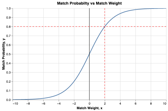
To make this usable, we take logs and get a weight score:

W = Σ [γᵢ log(mᵢ / uᵢ) + (1 − γᵢ) log((1 − mᵢ) / (1 − uᵢ))]

Interpretation:

• Agreement on a strong field → big positive weight
• Agreement on a weak field → small weight
• Disagreement on a reliable field → negative weight

The result is a single numeric score per record pair.

This is the thing people actually use.

Example (informal):

• Two records agree on date of birth and postcode, partially agree on name, and disagree on address.
• DOB agreement contributes a large positive weight, name a modest one, address a small negative.
• The total score still favours “match” — not because any field is decisive, but because the balance of evidence is.

Step 5: Where Do m and u Come From?

Of course, none of this works unless the model has reasonable estimates of how fields behave in practice. Fellegi–Sunter doesn’t assume these quantities are known — it provides a way to infer them from the data itself.

You don’t magically know mᵢ and uᵢ.

Fellegi–Sunter gives you two options.

Supervised

If you have labelled matches and non-matches:

• Estimate mᵢ and uᵢ directly from frequencies

Unsupervised (The Classic Approach)

If you don’t have labels (the usual case):

Use the Expectation–Maximization (EM) algorithm.

• E-step:
  Estimate the probability each pair belongs to M or U, given current parameters
• M-step:
  Re-estimate mᵢ and uᵢ using those probabilities
• Repeat until convergence

This works because the mixture proportions are highly imbalanced and the agreement patterns are sufficiently informative, aka:

• The dataset is large
• Non-matches massively outnumber matches

Which is almost always true.

Step 6: Decision Rules (Where Policy Enters)

Up to this point, everything has been about scoring and ranking uncertainty. But a scoring system on its own doesn’t make decisions. Turning weights into actions requires explicit choices about acceptable error.

Once every pair has a weight, you sort them and apply thresholds.

Fellegi–Sunter defines three regions:

• Above λ (upper threshold) → automatic Match
• Below μ (lower threshold) → automatic Non-match
• Between μ and λ → clerical review

Those thresholds are not statistical facts — they are policy choices.

They depend on:

• Cost of false positives
• Cost of false negatives
• Regulatory context
• Operational tolerance for error

This is where “pure math” ends and governance begins.

Why This Model Endures

Many record linkage techniques have come and gone, often tied to particular technologies or datasets. Fellegi–Sunter has lasted because its core assumptions align uncomfortably well with reality.

Fellegi–Sunter survives because it gets several things right that many modern approaches forget.

It treats uncertainty as fundamental

Not a failure mode.

It’s interpretable

You can explain why two records matched.

It’s flexible

Exact matches, fuzzy strings, categorical fields — all fit.

It works without labels

Which is still the default reality in many domains.

It scales (with blocking)

You reduce the O(n²) explosion by only comparing plausible candidates.

Where It Breaks (and How People Extend It)

Endurance does not mean perfection. The same simplifying assumptions that make Fellegi–Sunter usable also define its limits, and most modern work in this space is best understood as attempts to relax those assumptions.

Independence is a lie

Names, gender, and geography correlate.
Extensions model dependencies explicitly.

Binary agreement is crude

Modern systems use multi-level agreements or distance metrics.

Brute-force comparison doesn’t scale

Blocking, indexing, and partitioning are mandatory at scale.

Modern extensions include:

• Multi-file linkage
• Hybrid ML models
• Active learning with human feedback

But underneath, the logic is still recognisably Fellegi–Sunter.

Where You Actually See It Used

Despite being over half a century old, this model is not confined to textbooks or legacy systems. It continues to operate quietly underneath many large-scale, high-stakes data integration efforts.

• Census and population statistics
• Healthcare record linkage
• Financial services (KYC / AML / entity resolution)
• Customer deduplication in large platforms

Often without attribution.
Often buried under layers of tooling.
But it’s there.

The Bottom Line

The Fellegi–Sunter model isn’t just a historical curiosity.

It’s the moment record linkage stopped pretending that data is clean, identifiers are reliable, and matches are binary facts.

It formalised the idea that:

Matching is about weighing evidence under uncertainty, not enforcing rules.

Everything that came after is either:

• a refinement of that idea, or
• an attempt to hide it behind more compute.

And if you don’t understand Fellegi–Sunter, you don’t really understand record linkage — you’re just running code.

Appendix A: If You *Really* Want The Math

Everything so far has focused on intuition and consequences rather than derivations. For completeness — and for readers who want to see the machinery explicitly — this appendix lays out the formal expressions behind the narrative.

Everything above can be formalised. This is the machinery underneath the intuition.

Likelihood ratio

For a record pair with comparison vector
$\gamma = (\gamma_1, \gamma_2, \ldots, \gamma_k)$γ=(γ1​,γ2​,…,γk​),
the Fellegi–Sunter model computes a likelihood ratio:$$R = \frac{P(\gamma \mid M)}{P(\gamma \mid U)}$$R=P(γ∣U)P(γ∣M)​

Under the conditional independence assumption:$$R = \prod_{i=1}^{k} \frac{m_i^{\gamma_i}(1 – m_i)^{1 – \gamma_i}} {u_i^{\gamma_i}(1 – u_i)^{1 – \gamma_i}}$$R=i=1∏k​uiγi​​(1−ui​)1−γi​miγi​​(1−mi​)1−γi​​

where:

• $m_i = P(\text{agreement on field } i \mid M)$mi​=P(agreement on field i∣M)
• $u_i = P(\text{agreement on field } i \mid U)$ui​=P(agreement on field i∣U)

Log-weight form (what implementations actually use)

Taking logs gives an additive score:$$W = \sum_{i=1}^{k} \left[ \gamma_i \log\left(\frac{m_i}{u_i}\right) + (1 – \gamma_i)\log\left(\frac{1 – m_i}{1 – u_i}\right) \right]$$W=i=1∑k​[γi​log(ui​mi​​)+(1−γi​)log(1−ui​1−mi​​)]

This is the match weight:

• positive contributions from informative agreements
• negative contributions from unlikely disagreements

Thresholds on $W$W implement match / non-match / review decisions.

Estimating $m$m and $u$u (EM, in four lines)

When matches are not labelled:

1. Initialise $m_i, u_i$mi​,ui​ and the prior $P(M)$P(M)
2. E-step: estimate $P(M \mid \gamma)$P(M∣γ) for each pair using current parameters
3. M-step: re-estimate $m_i, u_i$mi​,ui​ from those expectations
4. Iterate until convergence

This works because non-matches vastly outnumber matches.

That’s it.
That’s the formal core.

If you understood the article without this section, you already understand Fellegi–Sunter.
If you didn’t… equations weren’t going to save you anyway.

Appendix B: Fellegi–Sunter Toy Example: Calculating Match Weights in Practice

This standalone example demonstrates how the Fellegi–Sunter model turns field-by-field agreements into a single numeric match weight. We use realistic (simplified) m and u probabilities and log base 2 for weights (common in implementations like Splink for interpretability in “bits of evidence”).

Step 1: Field Parameters

Field	mᵢ (prob agree if true match)	uᵢ (prob agree if non-match)	Agreement weight: log₂(mᵢ / uᵢ)	Disagreement weight: log₂((1-mᵢ) / (1-uᵢ))
First Name	0.90	0.0100	6.49	-3.31
Surname	0.95	0.0050	7.57	-4.31
DOB	0.98	0.0001	13.26	-5.64
Postcode	0.85	0.0010	9.73	-2.74
Gender	0.99	0.5000	0.99	-5.64

Step 2: Example Record Pairs

Pair A (likely a true match, e.g., person moved house): Agrees on First Name, Surname, DOB, Gender; disagrees on Postcode. Comparison vector γ: [1, 1, 1, 0, 1]

Match weight W = 6.49 + 7.57 + 13.26 + (-2.74) + 0.99 = +25.57 → Extremely strong evidence for match (rare agreements like DOB dominate).

Pair B (likely non-match): Agrees on Gender only; disagrees on everything else. Comparison vector γ: [0, 0, 0, 0, 1]

Match weight W = -3.31 + -4.31 + -5.64 + -2.74 + 0.99 = -15.02 → Strong evidence against match (disagreements on reliable fields hurt a lot).

This illustrates how the model weighs evidence: powerful positive boosts from informative agreements, penalties for unlikely disagreements, and little credit for common coincidences (like Gender).

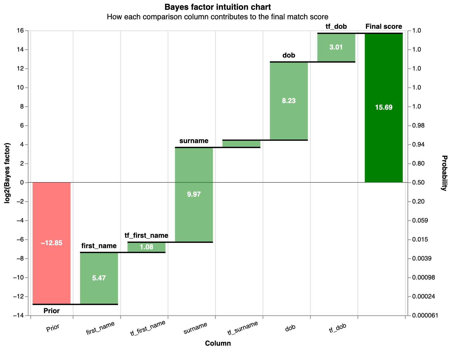
Visualising Match Weights in Real Tools

In practice, tools like Splink produce diagnostics like these:

moj-analytical-services.github.io

Term frequency adjustments – Splink

Waterfall chart showing how each field contributes to an individual pair’s match weight (from Splink docs).

moj-analytical-services.github.io

The Fellegi-Sunter Model – Splink

Typical score distribution: match weights form two overlapping but separable histograms (matches shift right).

moj-analytical-services.github.io

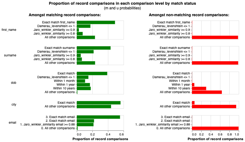
match weights chart – Splink

m/u parameter visualisation—shows how fields vary in discriminativeness.

These examples and visuals bring the Fellegi–Sunter model to life. You can reproduce similar results instantly in Splink’s interactive demos.

Appendix C: Practical Implementation Pointers

How to Try This Today

The Fellegi–Sunter model isn’t just theory—modern open-source tools implement it (and sensible extensions) out-of-the-box.

The best place to start is Splink (free, Python/SQL, developed by UK Ministry of Justice):

• Explicitly based on Fellegi–Sunter, with EM estimation, blocking, multi-level fuzzy comparisons, and term-frequency adjustments (to relax crude u-probabilities for common names).
• Scalable to billions of comparisons.
• Excellent diagnostics (waterfall charts explaining individual matches, match weight histograms).

Get started instantly:

• Interactive demos in your browser: https://moj-analytical-services.github.io/splink/demos/demos.html
• Full docs and tutorials: https://moj-analytical-services.github.io/splink/

Alternatives:

• fastLink (R package, very faithful to classic FS).
• Dedupe.io (Python, more ML-focused but still FS-inspired).

Run a toy dataset in Splink today… you’ll see m/u estimates, weights, and thresholds emerge automatically.